What Is a SFP 100km Transceiver? ER vs. ZR Technical Guide

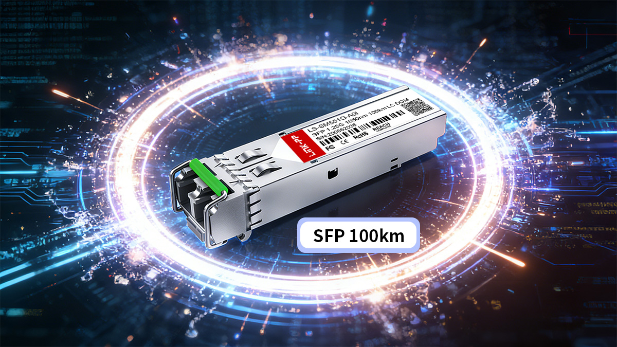
A SFP 100km transceiver is a long-reach optical module engineered for high-power transmission over single-mode fiber (SMF), typically operating in the 1550 nm low-attenuation window to support spans approaching 100 kilometers under controlled link conditions. These modules are commonly categorized as ER (Extended Reach) or ZR (80–100 km class) depending on optical budget, transmit power, receiver sensitivity, and standards alignment.

In 10 Gigabit Ethernet environments, long-reach optics are historically associated with specifications defined under IEEE 802.3ae, while higher-speed long-distance implementations relate to IEEE 802.3ba. However, it is important to distinguish between form factor, reach class, and standard compliance:

• Form factor (SFP+, XFP, QSFP, etc.) defines the physical module type.

• Reach designation (ER, ZR) describes the optical budget and target span.

• IEEE standard clauses define Ethernet PMD requirements at specific distances (e.g., 40 km for 10G ER).

Notably, “100km” is not a guaranteed transmission distance—it is a reach class based on nominal optical budget assumptions. Real-world performance depends on:

• Fiber attenuation (typically ~0.20–0.25 dB/km at 1550 nm for OS2 fiber)

• Connector and splice loss

• Chromatic dispersion

• System margin requirements

• Receiver overload threshold

Because of these variables, a 100km-rated transceiver may require optical amplification (such as EDFA) in certain deployments, while in clean, low-loss fiber environments it may operate unamplified. Engineering validation through link budget calculation is therefore mandatory.

This guide provides a structured technical analysis of:

• What defines a 100km SFP transceiver

• The difference between ER and ZR reach classes

• Optical budget calculation methodology

• Wavelength and laser technology used

• Amplification considerations

• Deployment risks and compatibility factors

The goal is to clarify engineering assumptions, eliminate common misconceptions, and provide standards-aligned deployment guidance for long-haul Ethernet optical links.

✅ What Is a SFP 100km Transceiver?

A SFP 100km transceiver is a high-power, long-reach optical module designed for transmission over single-mode fiber (SMF) in the 1550 nm low-attenuation window, engineered to provide an optical power budget typically in the ≥30 dB class, enabling spans approaching 100 km under controlled link conditions.

It is important to clarify that “100km” is a reach classification based on optical budget assumptions—not a guaranteed distance under all fiber conditions.

1. Designed for Single-Mode Fiber (SMF)

100km SFP modules are engineered exclusively for single-mode fiber, typically:

• ITU-T G.652.D compliant fiber

• OS2 low-attenuation outdoor fiber

• Core diameter ~9 µm

Multimode fiber (MMF) is not suitable due to modal dispersion and excessive attenuation at long distances.

At 1550 nm, modern OS2 fiber typically exhibits attenuation around:

• ~0.20–0.25 dB/km (field-dependent)

For a 100 km span, fiber attenuation alone may account for:

20–25 dB of loss (excluding connectors and splices)

This is why high optical budget design is mandatory.

2. Operation in the 1550 nm Low-Attenuation Window

100km transceivers operate in the 1550 nm region because:

• It offers the lowest attenuation in standard single-mode fiber

• It aligns with the C-band (approximately 1530–1565 nm)

• It is compatible with optical amplification technologies

Shorter wavelengths such as 850 nm or 1310 nm are not suitable for 100 km Ethernet spans due to higher attenuation and dispersion constraints.

The 1550 nm window is therefore the practical foundation for long-haul and metro long-reach optics.

3. High Transmit Power

To compensate for long fiber attenuation, 100km modules are designed with significantly higher launch power compared to short- or mid-reach optics.

Typical transmit output levels (implementation-dependent):

• Often in the positive dBm range

• Commonly between +2 dBm and +6 dBm for high-budget ZR-class optics

Exact values vary by manufacturer and reach class, and must always be verified on the module datasheet.

Higher transmit power directly increases the available optical budget, but also introduces considerations such as:

• Receiver overload at short distances

• Optical safety compliance

• Power balancing when amplification is used

4. High Receiver Sensitivity

In addition to higher transmit power, 100km SFP modules incorporate receivers with enhanced sensitivity.

Typical receiver sensitivity for long-reach 10G ZR-class optics:

• Often in the range of −24 dBm to −28 dBm (implementation-dependent)

High sensitivity allows detection of weak optical signals after long fiber attenuation.

However, this also means:

• Overload thresholds must be respected

• Optical attenuators may be required for short spans

Receiver overload is a common deployment issue when long-reach modules are used over short fiber distances.

5. SFP 100km Typical Use Cases

6. 100km transceiver Summary

A SFP 100km transceiver is defined by four core characteristics:

1. Operation over single-mode fiber

2. Use of the 1550 nm low-attenuation window

3. High transmit optical power

4. High receiver sensitivity

5. Optical budget typically in the ≥30 dB class

However, achieving 100 km in practice depends on disciplined link budget calculation, fiber quality, dispersion management, and proper system margin planning—not merely the label printed on the module.

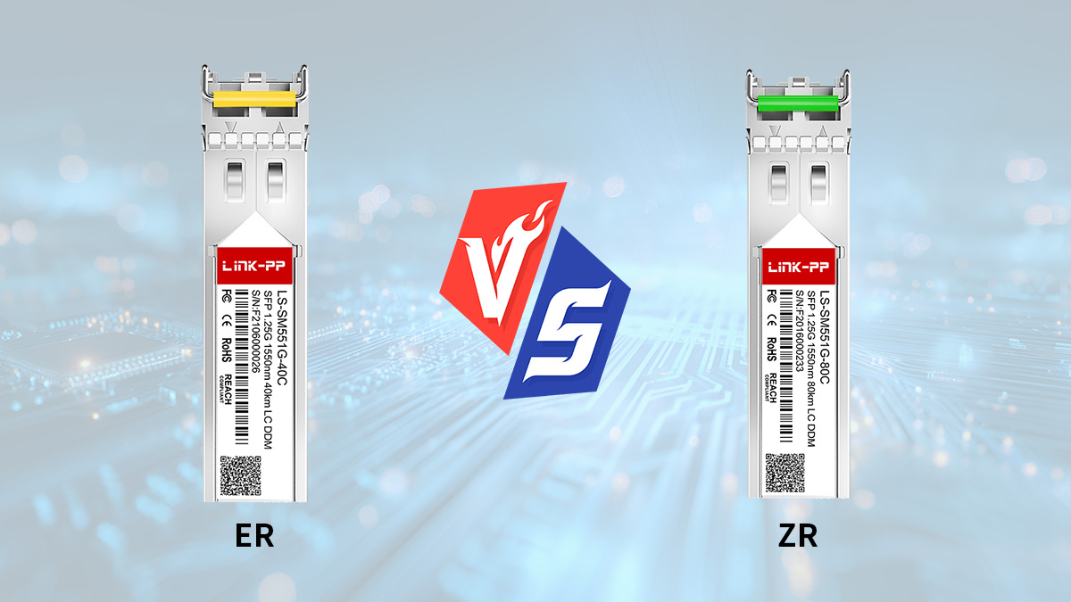
✅ SFP ER vs. ZR: What’s the Difference?

ER (Extended Reach) and ZR (80–100 km class) transceivers both operate in the 1550 nm window over single-mode fiber, but they differ significantly in standard definition, optical budget, and deployment assumptions. ER is formally defined in IEEE Ethernet specifications for ~40 km operation, while ZR is typically a higher-power industry extension targeting 80–100 km spans.

Standards Context

• 10GBASE-ER (40 km) is defined under IEEE 802.3ae.

• Higher-speed long-reach implementations relate to IEEE 802.3ba.

Important clarification:

• ER is explicitly standardized for 40 km in 10G Ethernet.

• “ZR” for 10G (80 km / 100 km class) is not defined as a separate IEEE clause; it is commonly implemented as a vendor-extended higher optical budget optic while maintaining Ethernet framing.

• At higher speeds (e.g., 100G), ZR terminology may align with different MSAs or coherent implementations, which are technically distinct from 10G direct-detect ZR optics.

ER vs. ZR Comparison

◆ Reach Definition

ER (Extended Reach)

• Designed for up to approximately 40 km over single-mode fiber

• Assumes controlled dispersion and attenuation

• Fully standardized under IEEE for 10GBASE-ER

ZR (Extended Extended Reach)

• Designed for longer spans, typically 80–100 km class

• Higher transmit power and/or improved receiver sensitivity

• Often implemented beyond strict IEEE PMD definitions (vendor-specific for 10G)

◆ Optical Budget Differences

Optical budget determines maximum allowable link loss:

Optical Budget = Minimum Tx Power − Receiver Sensitivity

Typical engineering ranges:

• ER: ~20–25 dB

• ZR: ~28–32 dB

That additional ~6–8 dB budget difference enables significantly longer span capability, assuming fiber attenuation around 0.20–0.25 dB/km at 1550 nm.

However, longer reach also increases:

• Chromatic dispersion accumulation

• Sensitivity to fiber quality

• Power balancing requirements

◆ Amplification Considerations

ER Deployment

• Typically deployed without optical amplification

• Direct point-to-point links within defined span

ZR Deployment

• May operate unamplified on low-loss fiber

• Often paired with EDFA amplification in longer or higher-loss spans

• More sensitive to dispersion over extended distances

Amplifier necessity depends on total span loss, not only nominal distance.

◆ Application Scope

ER Optics

• Metro aggregation

• Campus interconnection

• Enterprise long-distance links

ZR Optics

• Regional backbone

• Rural long-haul spans

• Inter-city connectivity

ZR optics are generally chosen when fiber spans exceed 40 km and infrastructure expansion is limited.

Difference Between ER and ZR Conclusion

The primary difference between ER and ZR lies in optical budget and deployment expectations, not wavelength.

• ER = standardized 40 km class with controlled parameters

• ZR = higher-power extended reach (80–100 km class), often vendor-defined in 10G environments

Selecting between ER and ZR requires accurate link budget calculation, dispersion evaluation, and consideration of amplification strategy—not simply distance estimation.

✅ Optical Budget and Link Engineering for 100km

A “100km” label on an SFP transceiver does not guarantee stable operation at 100 km. It indicates a target reach under nominal fiber conditions. Actual feasibility must be verified through disciplined optical link budget calculation.

Long-haul Ethernet design is fundamentally a power balance problem.

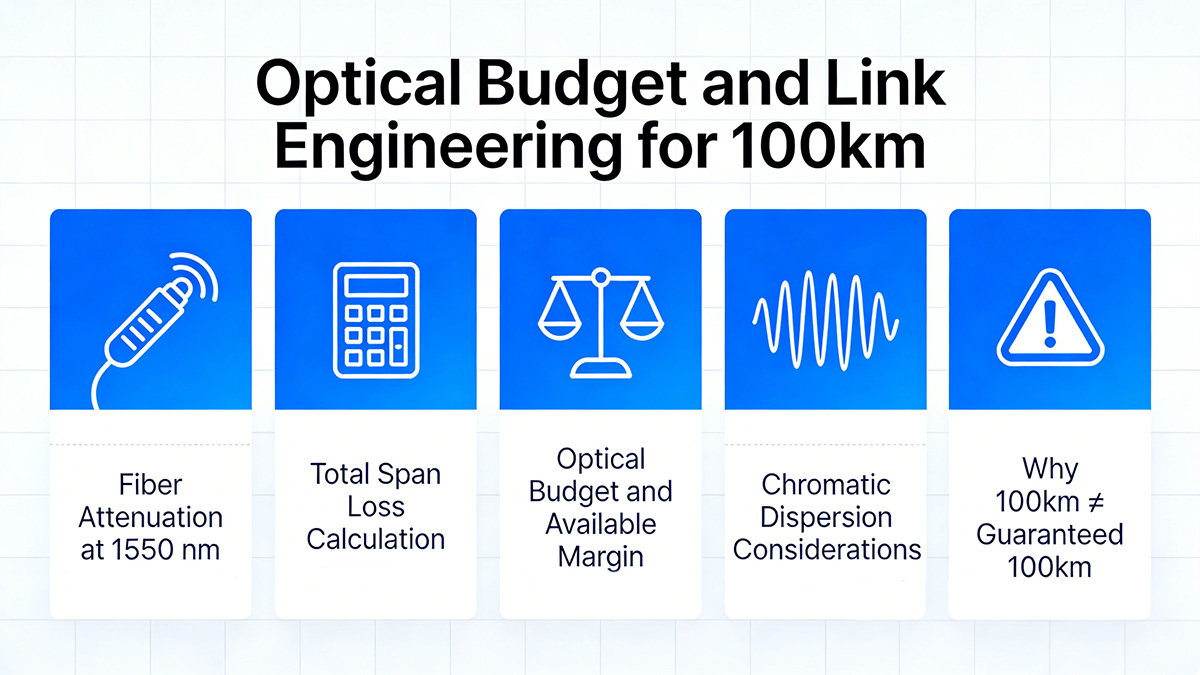
▶ Fiber Attenuation at 1550 nm

100km-class optics operate in the 1550 nm window because it offers the lowest attenuation in standard single-mode fiber.

Typical attenuation values for modern OS2 fiber:

• 0.20–0.25 dB/km @ 1550 nm

For a 100 km span:

• 0.20 dB/km → 20 dB fiber loss

• 0.25 dB/km → 25 dB fiber loss

This calculation excludes connectors, splices, and aging effects.

Even small deviations in fiber quality significantly affect long-haul feasibility.

▶ Total Span Loss Calculation

Total span loss must include all passive components, not just fiber distance.

Total Loss (dB) = Fiber Loss + Connector Loss + Splice Loss + Patch Panel Loss

Typical engineering assumptions:

• Connector pair: 0.5–1.0 dB (depending on quality and cleanliness)

• Fusion splice: ~0.05–0.1 dB per splice

• Patch panel / distribution frame: 0.5–1.0 dB

Example scenario (illustrative):

• 100 km fiber @ 0.22 dB/km → 22 dB

• 2 connector pairs → 1.0 dB

• 4 splices → 0.4 dB

Total span loss ≈ 23.4 dB

This value must be compared against the module’s optical budget.

▶ Optical Budget and Available Margin

Optical budget is determined by:

Optical Budget = Minimum Tx Power − Receiver Sensitivity

However, engineering validation requires margin calculation:

Available Margin = Tx Power − Total Loss − Receiver Sensitivity

If Available Margin ≤ 0 dB, the link will fail.

For production networks, recommended system margin:

• ≥ 3 dB minimum

• 5 dB preferred for long-haul reliability

This margin accounts for:

• Fiber aging

• Temperature variation

• Component drift

• Measurement uncertainty

▶ Chromatic Dispersion Considerations

At 1550 nm, chromatic dispersion in standard G.652 fiber is approximately:

• ~17 ps/nm·km

Over 100 km:

• ~1700 ps/nm accumulated dispersion

For 10G direct-detect systems, dispersion tolerance becomes an engineering constraint. Some 100km ZR-class optics rely on tighter laser spectral width and receiver tolerance to operate without external dispersion compensation.

Dispersion must be validated, especially beyond 80 km.

▶ Why 100km ≠ Guaranteed 100km

The printed reach rating assumes:

• Low-loss fiber (~0.20 dB/km)

• Minimal connectors

• Controlled dispersion

• Clean optical interfaces

Real-world conditions often differ.

A “100km” module deployed on:

• 0.25 dB/km fiber

• Multiple patch panels

• Aging splices

May only support 80–90 km reliably.

Conversely, extremely clean low-loss fiber may allow stable operation beyond nominal rating—but this should never be assumed without calculation.

▶ SFP 100km Notes:

Distance is not the design variable—optical loss and dispersion are.

For any 100km SFP deployment:

1. Calculate total span loss.

2. Compare against optical budget.

3. Confirm ≥3 dB system margin.

4. Validate dispersion tolerance.

Only after these steps can a 100 km link be considered technically justified.

✅ Does a 100km SFP Require Optical Amplification?

A SFP 100km transceiver is typically designed with a high optical budget (often ~28–32 dB class for ZR-type optics). Whether amplification is required depends on total span loss, dispersion, and system margin—not simply distance.

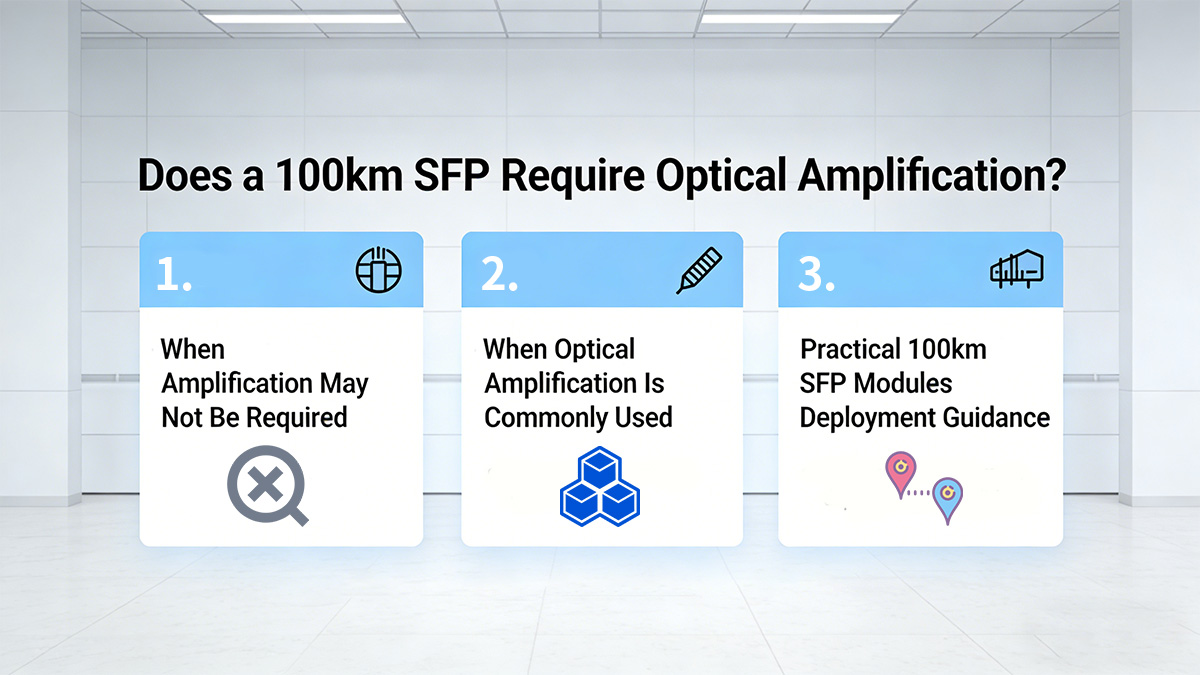
When Amplification May Not Be Required

In controlled conditions, a 100km SFP may operate without external amplification.

Typical favorable conditions:

• High-quality OS2 single-mode fiber

• Attenuation close to ~0.20 dB/km @1550 nm

• Minimal connector and splice loss

• Clean optical interfaces

• Adequate system margin (≥3 dB)

Example Link Budget Calculation (100 km)

In such cases, direct point-to-point operation may be feasible without amplification.

However, this assumes optimal fiber conditions.

When Optical Amplification Is Commonly Used

In practical long-haul deployments, amplification is frequently required due to:

• Higher fiber attenuation (~0.23–0.25 dB/km)

• Multiple patch panels

• Fiber aging

• Additional span elements (ODF, protection switching)

• Dispersion penalties

Amplification improves received signal strength and increases operational margin.

Common amplifier types include:

Booster Amplifier

• Installed immediately after the transmitter

• Increases launch power into the fiber

• Used when long spans require stronger initial signal

Pre-Amplifier

• Installed before the receiver

• Improves effective receiver sensitivity

• Used when signal arrives near sensitivity threshold

EDFA (Erbium-Doped Fiber Amplifier)

The most common long-haul amplification technology.

Key characteristics:

• Operates in the C-band (approximately 1530–1565 nm)

• Optimized for 1550 nm wavelength region

• Provides high gain with relatively low noise figure

• Compatible with DWDM systems

Because 100km SFP modules operate near 1550 nm, they align with the EDFA operating window.

Engineering Considerations with Amplification

Amplifiers introduce additional design variables:

• Gain must be carefully balanced

• Excess power may cause receiver overload

• Amplifier noise figure affects signal-to-noise ratio

• Power leveling may be required in multi-span systems

Improper amplification can degrade, not improve, link performance.

Practical 100km SFP Modules Deployment Guidance

Amplification is typically considered when:

• Total span loss approaches or exceeds optical budget

• System margin is <3 dB

• Network reliability requirements are high

• Fiber conditions are uncertain

In many metro-to-regional spans, at least one amplification stage is included for engineering safety—even if raw calculations suggest it may not be strictly required.

✅ Wavelength and Laser Type Used in 100km Modules

Long-reach 100km SFPs are defined by strict wavelength and laser requirements. At this distance class, wavelength stability, spectral purity, and dispersion tolerance become critical engineering factors.

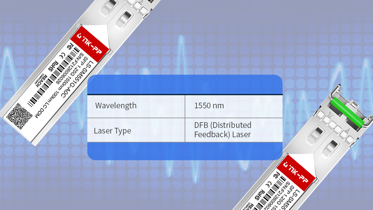
1. Operating Wavelength: 1550 nm Region

100km modules operate in the 1550 nm low-attenuation window of single-mode fiber.

Reasons:

• Lowest fiber attenuation (~0.20–0.25 dB/km for OS2)

• Alignment with the optical C-band (1530–1565 nm)

• Compatibility with EDFA amplification

• Better long-distance dispersion performance compared to 1310 nm at 10G long spans

While 1310 nm is suitable for shorter long-reach optics (e.g., 10 km / 20 km classes), it is not practical for 100 km direct-detect Ethernet spans due to attenuation and dispersion limitations.

Therefore, 100km-class SFP modules are engineered around the 1550 nm window.

2. Laser Type: DFB (Distributed Feedback) Laser

100km SFP modules use DFB (Distributed Feedback) lasers, not VCSEL technology.

Key characteristics of DFB lasers:

• Narrow spectral linewidth

• Stable wavelength output

• High optical output power

• Good dispersion tolerance

Narrow linewidth is essential because chromatic dispersion accumulates significantly over 100 km (~17 ps/nm·km in G.652 fiber). Broader spectral sources would experience excessive pulse broadening at this distance.

3. DWDM Grid Compliance (Common in ZR-Class Optics)

Many 100km modules—particularly ZR-class implementations—are designed to align with DWDM channel grids.

Typical characteristics:

• Fixed C-band wavelength

• ITU-T channel spacing (e.g., 100 GHz grid)

• Tight wavelength tolerance

DWDM compliance enables:

• Multi-channel long-haul transmission

• Compatibility with optical amplifiers

• Integration into metro or regional backbone systems

However, not all 100km SFP modules are full DWDM pluggables—some operate at fixed 1550 nm without multi-channel grid tuning. Datasheet verification is essential.

4. Spectral Width and Stability

For 100 km spans:

• Laser spectral width must be narrow

• Wavelength drift must be tightly controlled

• Temperature stabilization is required

Excessive spectral width increases dispersion penalty and reduces eye opening at the receiver.

DFB lasers are selected specifically to maintain performance under these constraints.

5. What 100km Modules Do NOT Use

To avoid common misconceptions:

• ❌ 100km modules do not use 850 nm (multimode short-reach wavelength)

• ❌ 100km modules do not use VCSEL lasers

VCSEL technology is optimized for:

• Short-reach multimode links

• 850 nm operation

• Data center distances (tens to hundreds of meters)

It is not suitable for 100 km single-mode transmission.

6. 100km SFP Wavelength and Laser Summary

A SFP 100km typically features:

• Operation in the 1550 nm C-band window

• A high-power, narrow-linewidth DFB laser

• Often DWDM-grid alignment

• Tight wavelength stability for dispersion control

Wavelength precision and laser quality are foundational to achieving long-haul performance. Without narrow spectral output and stable 1550 nm operation, 100 km transmission is not technically viable.

✅ 100km Transceiver Fiber Type Requirements

Long-distance SFP transceivers designed for 100 km operation impose strict fiber type requirements. Proper fiber selection is critical to achieving the specified optical budget, signal integrity, and reliable link performance.

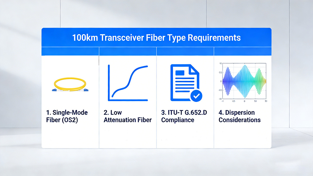
★ Single-Mode Fiber (OS2)

100 km SFP modules are engineered exclusively for single-mode fiber (SMF).

Key points:

• OS2 is the most common standard for long-haul terrestrial deployments.

• Core diameter: ~9 µm

• Cladding diameter: 125 µm

• Low macro- and micro-bend sensitivity

Single-mode fiber ensures minimal modal dispersion, which is essential for long spans where even small pulse broadening can significantly degrade the signal.

★ Low Attenuation Fiber

To support 100 km links without excessive amplification:

• Attenuation should be ≤0.25 dB/km at 1550 nm

• OS2 fiber typically provides 0.20–0.25 dB/km, depending on installation quality

• Connector and splice losses must be accounted for in the optical budget calculation

Exceeding attenuation budgets reduces system margin and may require additional amplification.

★ ITU-T G.652.D Compliance

100 km SFP transceivers require fibers compliant with G.652.D standard:

• Optimized for long-haul single-mode transmission

• Low chromatic dispersion in the 1550 nm window (~17 ps/nm·km)

• Reduced polarization mode dispersion (PMD)

• Compatible with EDFA amplification

G.652.D fibers are widely deployed in metro and regional backbone networks and are the default choice for high-reliability long-haul links.

★ Dispersion Considerations

Even with OS2/G.652.D fibers, chromatic dispersion accumulates over 100 km:

• 10G Ethernet: Moderate dispersion tolerance, often manageable without compensation

• 25G/100G links: Dispersion may become limiting; pre- or post-compensation modules could be required

• Narrow-linewidth DFB lasers mitigate pulse broadening

• DWDM deployment further emphasizes wavelength stability to avoid inter-channel crosstalk

To ensure reliable 100 km SFP operation:

1. Use OS2 single-mode fiber

2. Maintain low attenuation ≤0.25 dB/km

3. Ensure G.652.D compliance for dispersion and PMD control

4. Account for connector/splice losses in optical budget

5. Verify dispersion margin based on data rate and link design

Meeting these fiber requirements is essential; any deviation increases the likelihood of signal degradation, optical margin loss, or the need for amplification.

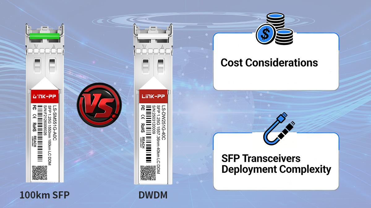
✅ When to Choose 100km SFP vs. DWDM Coherent Modules

Selecting the appropriate optical module for long-haul transmission requires careful evaluation of reach, data rate, network complexity, and cost. For spans around 100 km, network engineers often compare 100 km SFP/ZR-class modules with DWDM coherent 100G or higher modules.

10G ZR-Class SFP vs. 100G Coherent DWDM

Implication: ZR-class 10G modules are ideal for simpler point-to-point links, whereas coherent DWDM is suited for high-capacity backbone networks.

Cost Considerations

• 100 km SFP/ZR modules: Lower capital expenditure (CAPEX) and simpler operational expenditure (OPEX)

• 100G coherent DWDM: Higher CAPEX due to complex transceiver optics, DSP, and necessary ROADMs; OPEX also higher because of monitoring and wavelength management

Organizations must weigh link requirements vs. budget.

SFP Transceivers Deployment Complexity

• 100 km SFP: Plug-and-play, minimal configuration, works over standard OS2 fiber with optional EDFA

• DWDM coherent: Requires wavelength planning, network provisioning, ROADMs (Reconfigurable Optical Add-Drop Multiplexers), and link monitoring

Complex topologies favor coherent DWDM for scalability and capacity aggregation.

Choose 100 km SFP/ZR-class if:

• Data rate requirement is ≤10G

• Single point-to-point link

• Minimal operational complexity is desired

• Budget constraints exist

Choose DWDM coherent modules if:

• Data rates ≥100G

• Multi-channel backbone network

• ROADM integration required

• Advanced dispersion and OSNR management necessary

For long-haul spans up to 100 km:

• ZR-class SFP provides cost-effective, low-complexity solutions for moderate data rates

• Coherent DWDM modules are justified for ultra-high-capacity links with multiple wavelengths and advanced routing

Correct selection ensures optimized network performance, minimal margin loss, and controlled operational cost.

✅ SFP 100km Deployment Risks & Compatibility & EEPROM Considerations

Deploying 100 km SFP transceivers requires careful attention to link engineering, fiber condition, and module compatibility. Even with correctly specified modules, several risks can degrade performance or prevent successful operation.

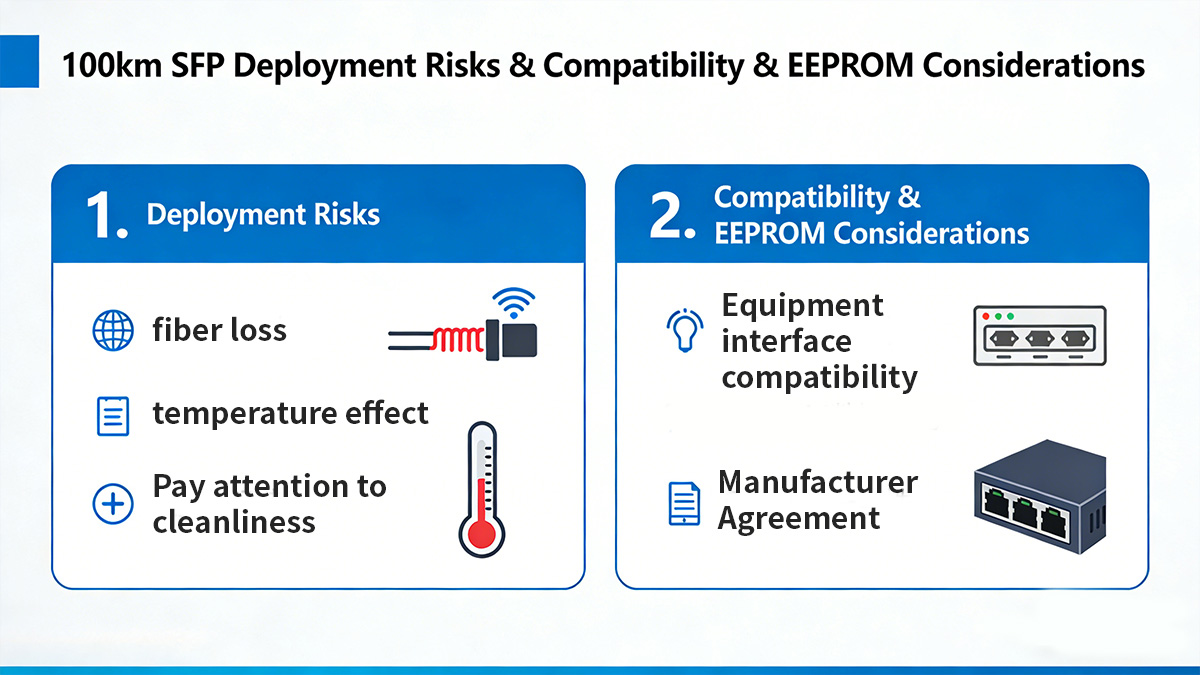
▲ Deployment Risks

▲ Compatibility & EEPROM Considerations

100 km SFPs rely on EEPROM identification and firmware compliance to ensure the host device accepts the module and monitors its operation correctly.

• Key References: SFF-8472

• DOM Monitoring: Provides real-time optical power, temperature, and voltage feedback

• Vendor Lock & Firmware Rejection: Some devices reject third-party modules based on EEPROM fields (Vendor OUI, part number, wavelength)

• Best Practice: Always verify EEPROM coding, cross-check compatibility lists, and update firmware if necessary

Engineering Note:

Accurate link budget calculation, DOM monitoring, and vendor-verified compatibility are essential for reliable 100 km SFP deployment. Ignoring these factors can lead to err-disabled interfaces, degraded signal quality, or reduced system margin.

✅ 100km Transceiver FAQs

Q1: Can 100km optics run at 50km?

Yes, they can operate over shorter distances, but the receiver may experience overload. Use an inline attenuator if necessary.

Q2: What happens if Rx power is too high?

Excessive optical power can saturate the receiver, causing signal errors or link instability. Attenuation or lower-power modules may be required.

Q3: Can I mix ER and ZR?

No, ER and ZR modules have different optical budgets. Mixing may cause link failure or margin loss.

Q4: Is dispersion compensation required?

For 10G ZR-class over OS2 fiber, usually not required. For higher-speed links or poor-quality fiber, dispersion compensation may be needed.

Q5: What is a 100km SFP transceiver?

A pluggable module designed for single-mode fiber over 100 km using 1550nm DFB lasers and high Rx sensitivity, typically with ≥30 dB optical budget.

Q6: Does 100km require optical amplification?

Depends on fiber and margin. Clean OS2 fiber may not need EDFA, but most real-world deployments use booster or pre-amplifiers.

Q7: What wavelength is used for 100km?

Typically 1550nm, within the C-band low-attenuation window. VCSELs or 850nm are not used.

Q8: What is the difference between ER and ZR?

Q9: Can a 100km module run without EDFA?

Yes, if fiber is low-loss OS2 and link margin is sufficient, amplification may not be necessary.

Q10: What fiber type is required?

Single-mode OS2 fiber, low attenuation, G.652.D compliant, with minimal splices and proper connector quality.

Q11: What is the optical budget of a 100km SFP?

Typically ≥30 dB, including Tx power, fiber loss, connector/splice loss, and required system margin.

✅ SFP 100km Transceiver Conclusion & Deployment Guidance

100 km SFP transceivers represent high-power, long-reach optical links that require careful engineering design and planning. Successful deployment depends on accurate link budget calculation, proper fiber type selection (SMF/OS2), and ensuring operation within the 1550nm low-attenuation window.

For most real-world scenarios, it is recommended to maintain at least 3 dB system margin to account for fiber aging, connector/splice losses, and potential variations in transmitter/receiver performance.

Deployment Guidance Highlights:

• Verify ER vs. ZR classification and optical budget

• Confirm fiber condition, splices, and connectors

• Monitor DOM readings for Tx/Rx power and temperature

• Ensure EEPROM and firmware compatibility

• Plan for amplification only if link loss exceeds module specifications

Explore LINK-PP’s full range of 100 km SFP transceivers for reliable long-haul connectivity. Ensure optimal deployment with engineer-verified modules, accurate link budgets, and full DOM support.

🔗 LINK-PP Official Store