
In modern fiber optic networks, ensuring a reliable connection between devices requires more than just plugging in a transceiver. One of the most critical factors determining whether a link operates flawlessly is the optical link budget. For SFP and SFP+ modules, the link budget defines the maximum allowable optical signal loss between the transmitter and receiver, ensuring data is transmitted with minimal errors.
At its core, the optical link budget is calculated as the difference between the minimum transmitter power and the minimum receiver sensitivity, typically measured in decibels (dB). However, real-world deployments introduce additional factors such as fiber attenuation, connector and splice losses, and a safety margin to account for aging components or installation imperfections. If the total link loss exceeds the link budget, the fiber connection may become unstable, leading to intermittent errors or complete link failure.
By understanding and accurately calculating the optical link budget, engineers and network designers can optimize their SFP deployments, select the right modules for specific fiber types, and troubleshoot connectivity issues efficiently. In this article, we’ll break down the calculation formula, the key loss components, a step-by-step example, and practical tips for achieving a robust fiber link.
Through this guide, you’ll gain the knowledge to ensure reliable SFP-based fiber connections, improve network stability, and make informed decisions when planning or upgrading fiber networks.
🟦 What Is Optical Link Budget in SFP Modules?
The optical link budget in SFP modules refers to the total amount of optical power loss (measured in dB) that a fiber optic link can tolerate while still maintaining reliable communication between the transmitter and receiver. In simple terms, it represents the power “allowance” available to overcome all losses in a fiber connection, including fiber attenuation, connectors, and splices.
At the device level, every SFP or SFP+ module has a defined range of optical output power (transmitter side) and required input sensitivity (receiver side). The difference between these two values defines the maximum usable signal loss that the link can support. If the total loss in the fiber system exceeds this budget, the signal becomes too weak, resulting in packet loss, unstable links, or complete failure.

Simple Definition
Optical Link Budget = Maximum allowable optical loss between an SFP transmitter and receiver while maintaining a stable fiber connection.
It is typically expressed in decibels (dB) and determines how far and how reliably an optical signal can travel through a fiber network.
Why Optical Link Budget Is Critical in SFP / SFP+ Networks
In real-world fiber deployments, SFP modules are used across enterprise switches, data centers, telecom networks, and industrial systems. In these environments, the optical link budget is critical because it directly determines:
Whether a 1G, 10G, or higher-speed link will establish successfully
How much fiber loss (distance + components) the system can tolerate
The stability and error rate of long-term data transmission
Even if two SFP modules are physically compatible, the link may still fail if the optical budget is insufficient for the installed fiber path.
Relationship Between Transmitter, Fiber, and Receiver
A fiber optic link can be understood as a power flow system:
Transmitter (Tx): Generates optical power (signal strength)
Fiber link: Introduces loss due to distance and physical components
Receiver (Rx): Requires a minimum optical power to correctly decode data
The optical link budget acts as the bridge between these three elements, ensuring that:
Tx power − Total fiber losses ≥ Rx sensitivity
If this condition is not met, the receiver cannot reliably interpret the incoming signal.
Why “Distance Rating” Alone Is Misleading
A common misconception in fiber networking is assuming that an SFP module’s distance rating (e.g., 10 km, 20 km) guarantees performance over that range. In reality, distance is only an approximation based on ideal fiber conditions and does not account for real deployment losses.
In practice, the actual performance depends on:
Fiber quality (OS2 vs. OM3/OM4)
Number of connectors and patch panels
Splice quality and quantity
Signal degradation over installation conditions
System safety margin requirements
This is why two identical “10km SFP modules” can perform very differently in different network environments. The optical link budget, not the labeled distance, is the true engineering constraint.
Optical link budget Summary
Optical link budget defines maximum allowable signal loss (dB) in SFP fiber links
It is determined by Tx power, Rx sensitivity, and total fiber system losses
It ensures stable communication across SFP/SFP+ optical networks
Distance ratings are estimates, not guarantees, making link budget calculation essential
🟦 Optical Link Budget Calculation Formula Explained
The optical link budget calculation formula is the foundation of all fiber optic power planning for SFP and SFP+ modules. It determines the maximum allowable signal loss a fiber link can tolerate while still maintaining reliable communication between devices.
Main Fiber Link Budget Formula
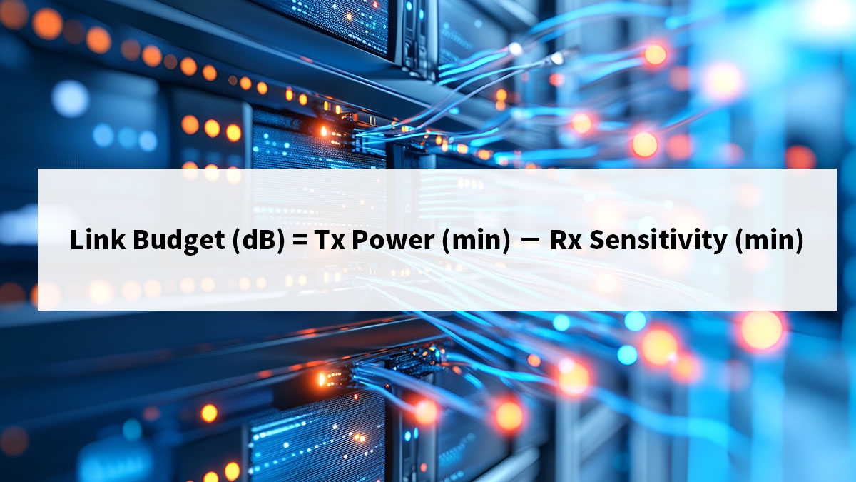
Link Budget (dB) = Tx Power (min) − Rx Sensitivity (min)
This formula defines the maximum optical loss threshold of a fiber optic system. If total losses in the fiber path exceed this value, the link will fail or become unstable.
Explanation of Each Variable
To correctly perform an optical link budget calculation, it is essential to understand each parameter in the formula:
1. Transmitter Power (Tx Power, dBm)
Represents the optical output power generated by the SFP transmitter
Measured in decibel-milliwatts (dBm)
Datasheets usually provide a range (e.g., max and min values)
For engineering design, the minimum Tx power must be used because it represents the worst-case output scenario.
2. Receiver Sensitivity (Rx Sensitivity, dBm)
Represents the minimum optical power required by the receiver to correctly decode data
Also measured in dBm
Lower (more negative) values indicate better sensitivity
The more sensitive the receiver, the more loss the system can tolerate.
Why Worst-Case Values Must Be Used
In real-world fiber network design, using typical or average values can lead to critical deployment failures. Professional network engineers always apply worst-case design rules, meaning:
Use minimum transmitter power, not typical power
Use minimum receiver sensitivity specification (worst-case threshold)
Account for manufacturing tolerances across different SFP batches
Why Optical Link Budget Calculation Matters in Real Deployments
SFP modules from different vendors—or even different production batches—can vary slightly within specification limits. If calculations are based on optimistic values, the system may appear functional in testing but fail under:
Temperature variation
Aging of optical components
Connector contamination or wear
Long-term signal degradation
Using worst-case values ensures the optical link budget represents a guaranteed operational boundary, not an ideal condition. This is critical in:
Data centers
Telecom backbone networks
Industrial fiber systems
High-reliability enterprise networks
key Takeway
Optical link budget is calculated using Tx power (min) − Rx sensitivity (min)
Tx power defines the output signal strength of the SFP transmitter
Rx sensitivity defines the minimum required input signal for decoding data
Worst-case values must always be used to ensure real-world deployment reliability
This formula is the foundation of all SFP fiber network power planning
🟦 Components of Fiber Optic Loss in Link Budget
In any optical link budget calculation for SFP modules, the total signal loss is not caused by fiber distance alone. Instead, it is the sum of multiple physical and installation-related losses that occur throughout the optical path.
Understanding these components is essential for accurate planning, troubleshooting, and ensuring long-term network stability.
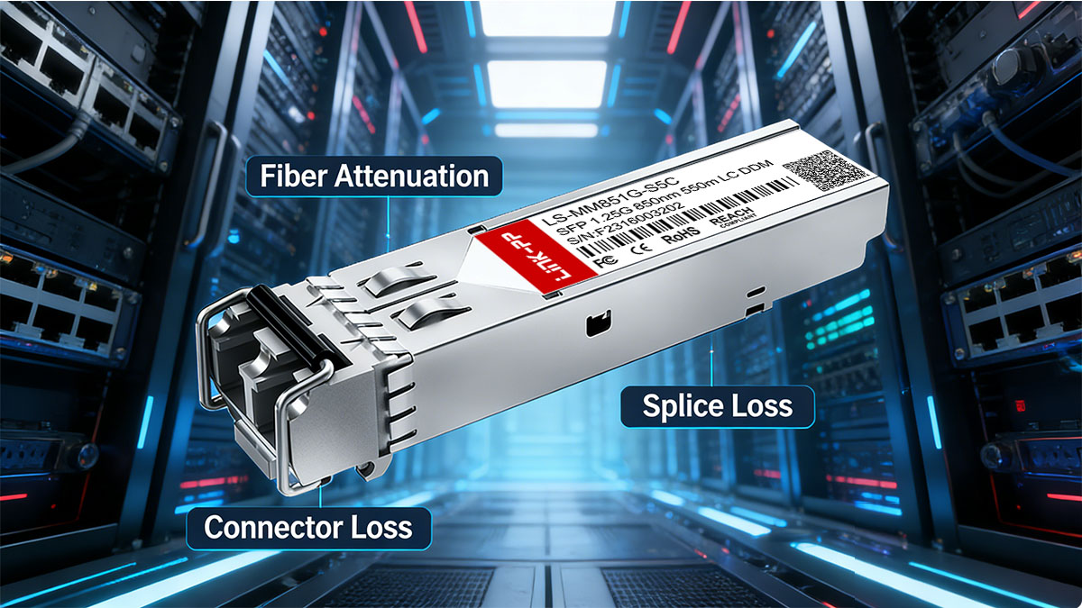
Key Components of Optical Loss in Fiber Links
Loss Component | Typical Value | Description | Impact on Link Budget |
|---|---|---|---|
Fiber Attenuation | ~0.35 dB/km @1310nm (SMF) | Signal loss as light travels through fiber over distance | Increases proportionally with distance |
Connector Loss | ~0.2–0.5 dB per connector pair | Loss introduced at each physical fiber connection | Accumulates with patch panels and couplers |
Splice Loss | ~0.1 dB per splice | Loss at fusion or mechanical splices | Usually small but additive in long links |
Safety Margin | 3–5 dB (recommended) | Design buffer for aging, dust, bending, repairs | Ensures long-term reliability |
Fiber Attenuation (Distance-Based Loss)
Fiber attenuation is the gradual reduction of optical signal strength as light travels through the fiber cable.
For Single-Mode Fiber (SMF) at 1310 nm, the typical attenuation is:
≈ 0.35 dB per kilometer
For longer wavelengths (e.g., 1550 nm), attenuation may be lower (~0.2 dB/km)
This means distance directly increases total optical loss, making it a major factor in long-range SFP deployments.
Connector Loss (Interface Loss)
Every time a fiber connection is made—such as through patch panels, adapters, or SFP ports—some signal is lost.
Typical loss per connector pair:
0.2 to 0.5 dB
Causes include:
Misalignment of fiber cores
Dust or contamination
Surface reflection
Even small connector losses can significantly reduce margin in borderline link budgets.
Splice Loss (Permanent Joint Loss)
Splices are used to permanently join fiber cables, usually in backbone or outdoor installations.
Typical splice loss:
~0.1 dB per splice
Types:
Fusion splicing (lower loss, more stable)
Mechanical splicing (slightly higher loss)
While small individually, multiple splices can accumulate in long-distance networks.
Safety Margin
The safety margin is a critical but often overlooked component in optical link budget design.
Recommended value:
3–5 dB
Purpose:
Compensate for fiber aging
Handle future repairs or modifications
Absorb unexpected losses (bending, contamination, temperature variation)
Without a safety margin, a link that initially works may become unstable over time.
Engineering Insight
In professional fiber design, the total optical loss is calculated as:
Total Loss = Fiber Attenuation + Connector Loss + Splice Loss + Safety Margin
A link is considered valid only when:
Link Budget ≥ Total Loss
This ensures the system operates reliably not only at installation, but throughout its lifecycle.
Fiber attenuation causes distance-based signal loss (~0.35 dB/km @1310nm SMF)
Connector loss occurs at every fiber interface (0.2–0.5 dB per pair)
Splice loss is minimal but accumulates (~0.1 dB per splice)
A 3–5 dB safety margin is required for real-world reliability
Total loss must always remain below the optical link budget threshold
🟦 Step-by-Step Optical Link Budget Calculation Example (10G SFP+)
To fully understand optical link budget calculation in real deployments, it is essential to walk through a practical engineering example. This section provides a worked calculation for a 10G SFP+ 10km single-mode fiber link, structured in a way that is easy to follow, verify, and cite in technical documentation.
Example Scenario: 10G SFP+ 10km Fiber Link
We will calculate whether the optical link is valid based on real-world loss components.
Given Conditions:
Fiber type: Single-mode fiber (SMF, OS2)
Distance: 10 km
Module: 10G SFP+ (LR class typical use case)
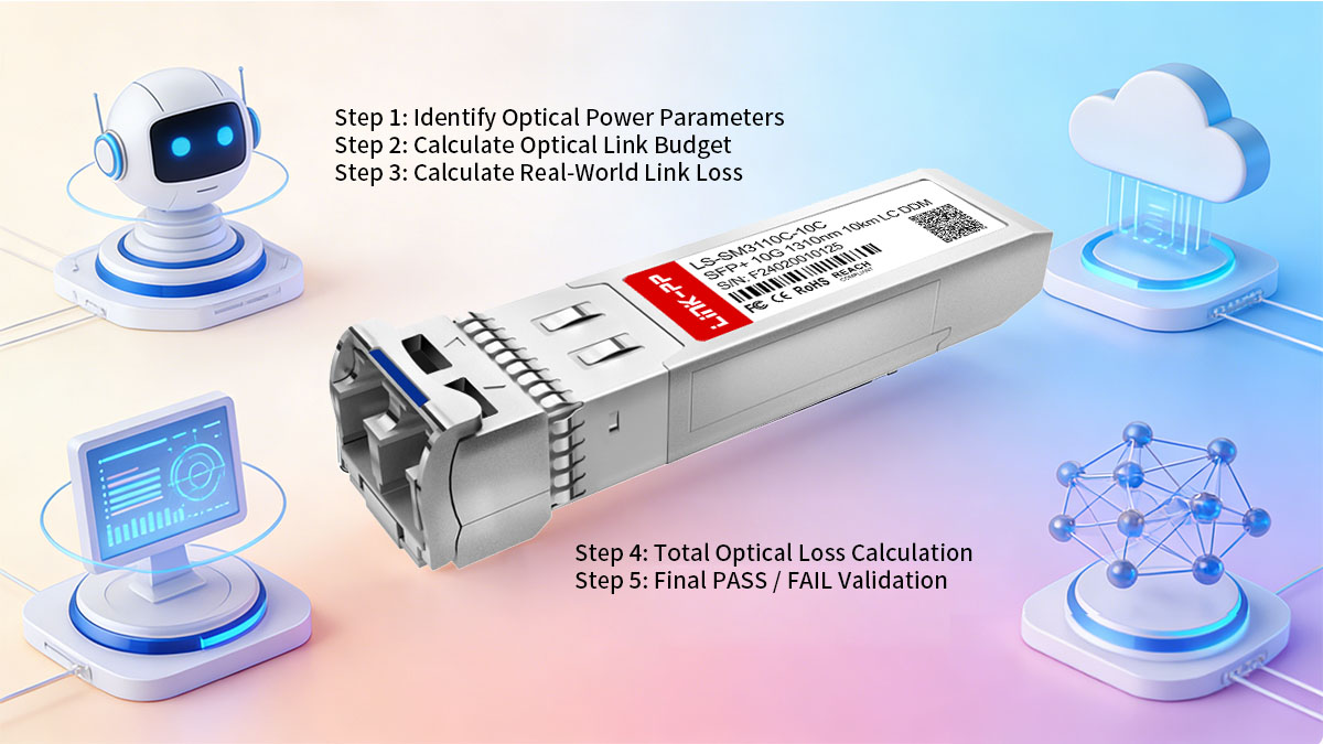
Step 1: Identify Optical Power Parameters
Transmitter Power (Tx)
Minimum Tx power: -8 dBm
Receiver Sensitivity (Rx)
Minimum Rx sensitivity: -16 dBm
Step 2: Calculate Optical Link Budget
Using the standard formula:
Link Budget = Tx(min) − Rx(sensitivity)
Link Budget=(−8)−(−16)=8 dBtext{Link Budget} = (-8) – (-16) = 8 text{ dB}Link Budget=(−8)−(−16)=8 dB
✔️ Available Optical Budget:
8 dB total allowable loss
Step 3: Calculate Real-World Link Loss
Now we calculate all real optical losses in the system.
3.1 Fiber Attenuation Loss
Typical SMF loss at 1310nm:
0.35 dB/km
0.35×10=3.5 dB0.35 times 10 = 3.5 text{ dB}0.35×10=3.5 dB
✔️ Fiber loss = 3.5 dB
3.2 Connector Loss
Assume:
2 connector pairs (Tx side + Rx side)
0.5 dB per connector pair
2×0.5=1.0 dB2 times 0.5 = 1.0 text{ dB}2×0.5=1.0 dB
✔️ Connector loss = 1.0 dB
3.3 Splice Loss
Assume:
2 splices in the route
0.1 dB per splice
2×0.1=0.2 dB2 times 0.1 = 0.2 text{ dB}2×0.1=0.2 dB
✔️ Splice loss = 0.2 dB
3.4 Safety Margin
Industry recommended margin:
3 dB
✔️ Safety margin = 3.0 dB
Step 4: Total Optical Loss Calculation
Total Loss=3.5+1.0+0.2+3.0
Total Loss=7.7 dB
Step 5: Final PASS / FAIL Validation
Compare:
Parameter | Value |
|---|---|
Optical Link Budget | 8 dB |
Total Loss | 7.7 dB |
✔️ Final Result:
8 dB (Budget) > 7.7 dB (Loss)
LINK STATUS: PASS (Valid and stable connection)
Engineering Interpretation
This result means:
The SFP+ link operates within safe optical power limits
Even with fiber attenuation and connector loss, signal remains stable
The 3 dB safety margin ensures long-term reliability
However, this is a borderline-efficient design, meaning:
Any additional connector
Dirty fiber ends
Cable bending or aging
could reduce the margin and push the link into failure conditions.
Optical link budget defines maximum allowable signal loss in SFP links
Example 10G SFP+ link budget = 8 dB (Tx − Rx calculation)
Total loss includes:
fiber attenuation (distance-based)
connector loss
splice loss
safety margin
Link is valid when budget > total loss
Real-world design must always include 3–5 dB safety margin
🟦 Optical Link Budget vs. Real-World Deployment Issues
While optical link budget calculation provides a precise engineering model for fiber design, real-world deployments often behave differently. In practice, many SFP and SFP+ link issues occur not because the theoretical budget is incorrect, but because real installation conditions introduce additional, unplanned losses.
This gap between theory and reality is one of the most common reasons for unstable fiber links, intermittent disconnections, or unexpected link failure in production networks.

Why Theoretical Budget Differs from Real Deployment
In an ideal calculation, all parameters (Tx power, Rx sensitivity, fiber loss) are stable and predictable. However, real environments introduce variability such as:
Manufacturing tolerance differences between SFP modules
Installation quality variations
Environmental stress (temperature, vibration)
Aging of connectors and fiber components
As a result, a link that appears “valid on paper” may operate near or below the real performance threshold in the field.
Dirty Connectors and Insertion Loss (Most Common Issue)
One of the most frequently reported real-world causes of link failure (also widely discussed in networking communities such as Reddit) is connector contamination.
How it affects link budget:
Dust or oil on fiber ends increases insertion loss
Even microscopic contamination can add 0.5–3 dB unexpected loss
Repeated reconnections worsen surface degradation
Practical insight:
Many “mysterious SFP failures” are resolved simply by cleaning LC connectors or replacing patch cords.
Fiber Bending and Aging Effects
Fiber optic cables are sensitive to physical stress.
Key issues include:
Macro-bending loss (tight cable bends)
Micro-bending loss (pressure from cable ties or trays)
Material degradation over time
Impact on link budget:
Additional unplanned attenuation
Can reduce available margin below safe threshold
Often intermittent and hard to diagnose
This is especially critical in high-density data center cabling environments.
Misinterpretation of “Distance Rating”
A common engineering misconception is assuming that:
“A 10 km SFP module will always work up to 10 km”
However, in real deployments:
Distance rating does NOT guarantee performance because it ignores:
Connector count
Patch panel loss
Splice quality
Fiber type variations (OS2 vs. mixed installations)
Environmental conditions
Engineering truth: Distance is a marketing approximation — link budget is the real design rule.
Importance of DOM (Digital Optical Monitoring)
Modern SFP and SFP+ modules often include DOM (Digital Optical Monitoring), which is critical for real-world troubleshooting.
What DOM provides:
Real-time Tx power
Real-time Rx power
Temperature monitoring
Voltage monitoring
Why DOM is essential in deployment:
DOM allows engineers to:
Detect margin degradation before failure
Identify dirty connectors (low Rx power)
Spot failing fiber runs or weak Tx modules
Compare expected vs. actual optical performance
TIPS:
In professional fiber network design, the key difference between stable and unstable links is not the formula itself, but:
How much real-world loss exceeds the calculated optical link budget margin
Experienced engineers always:
Design with 3–5 dB safety margin
Verify performance using DOM readings
Treat distance ratings as secondary reference only
Prioritize real measured optical power over theoretical assumptions
Real-world fiber links often deviate from theoretical optical link budget calculations
Dirty connectors can introduce significant insertion loss and link instability
Fiber bending and aging reduce actual signal strength over time
Distance ratings are not reliable design parameters compared to link budget analysis
DOM monitoring is essential for validating real optical power levels in SFP networks
🟦 How to Optimize Optical Link Budget for SFP Networks
Optimizing the optical link budget in SFP and SFP+ networks is essential for ensuring stable, long-term fiber performance. While correct calculation defines whether a link can work, optimization determines whether it will remain reliable under real-world conditions, aging, and environmental changes.
This section provides a practical engineering checklist used in real deployments to maximize link stability and reduce optical loss.

1. Match SFP Module Type (LR / SR / ER)
The first and most important optimization step is selecting the correct SFP optical class based on fiber type and distance requirements.
Common module types:
SR (Short Range) → Multimode fiber (MMF, OM3/OM4), short distance
LR (Long Range) → Single-mode fiber (SMF, up to ~10 km)
ER (Extended Range) → Long-distance SMF links (typically 40 km or more)
Optimization principle: Always match optical power class + fiber type + distance requirement to avoid wasted margin or link failure.
2. Reduce Connector Count (Minimize Insertion Loss)
Each connector introduces measurable signal loss, which directly reduces the available link budget.
Typical impact:
0.2–0.5 dB loss per connector pair
Optimization strategies:
Avoid unnecessary patch panels
Use direct fiber runs where possible
Consolidate cross-connect points
Maintain clean LC/SC interfaces
Fewer connection points = higher optical margin + better long-term stability
3. Use High-Quality Single-Mode Fiber (OS2)
Fiber quality significantly impacts attenuation and long-distance performance.
Recommended fiber:
OS2 Single-Mode Fiber
Benefits:
Lower attenuation (~0.35 dB/km at 1310 nm)
Better long-distance performance
More stable optical transmission
Avoid:
Mixed fiber types (MMF + SMF transitions)
Low-grade or aging cable infrastructure
4. Improve Installation Practices
Even correctly calculated link budgets can fail due to poor installation quality.
Best practices:
Ensure proper fiber cleaning before connection
Avoid tight bends (prevent macro-bending loss)
Maintain proper cable radius
Use certified termination tools and splicing equipment
Real-world insight: Installation quality often has more impact on link stability than theoretical optical design.
5. Maintain Safety Margin for Long-Term Reliability
The safety margin is one of the most critical yet frequently underestimated optimization factors.
Recommended margin:
3–5 dB minimum
Why it matters:
Compensates for:
Connector aging
Dust accumulation
Temperature variation
Future network expansion
Repair-related insertion loss
Engineering principle: A link without margin is a link designed for failure under real-world conditions.
In professional fiber network design, optimization is not just about meeting the link budget—it is about protecting margin over time.
A robust SFP network design follows this rule:
Available Link Budget − Total Loss ≥ Safety Margin
If this condition is not satisfied, the link may function initially but will degrade under real operational stress.
Match SFP modules correctly: SR (MMF), LR/ER (SMF)
Reduce connector count to minimize insertion loss
Use OS2 single-mode fiber for long-distance reliability
Follow proper installation practices to avoid hidden losses
Always maintain a 3–5 dB safety margin for long-term stability
Optimization ensures not only connectivity, but network durability and resilience
🟦 Common Optical Link Budget Mistakes Engineers Make
Even experienced network engineers can make mistakes when performing optical link budget calculations for optical modules. These errors often lead to unstable fiber links, unexpected downtime, or misleading assumptions about network capacity.
Understanding these common pitfalls is essential for building accurate, reliable, and production-grade fiber optic networks.
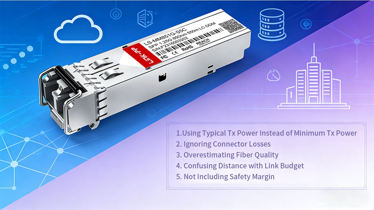
▶ Using Typical Tx Power Instead of Minimum Tx Power
One of the most critical calculation errors is using typical transmitter power values instead of minimum guaranteed values from the datasheet.
Why this is a problem:
Optical transmit power varies by manufacturing tolerance
“Typical” values represent average performance, not worst-case conditions
Real-world modules may operate closer to minimum specification
Always use minimum Tx power and minimum Rx sensitivity for link budget calculations.
This ensures the design remains valid under worst-case scenarios.
▶ Ignoring Connector Losses
Connector loss is often underestimated or completely omitted in simplified designs.
Typical reality:
Each connector pair: 0.2–0.5 dB loss
Multiple patch points significantly accumulate loss
Common mistake:
Calculating only fiber attenuation (km-based loss)
Ignoring patch panels and cross-connects
Impact: Even a few missed connectors can consume the entire safety margin in a marginal link.
▶ Overestimating Fiber Quality
Not all fiber is equal, and real-world fiber conditions often differ from ideal specifications.
Common issues:
Aging fiber with increased attenuation
Mixed fiber types (OS2 + legacy cabling)
Poor splicing quality in older infrastructure
Environmental stress affecting cable performance
Key insight: Engineers often assume “standard attenuation values,” but real installations frequently exceed them.
This leads to underestimated total link loss.
▶ Confusing Distance with Link Budget
This is one of the most widespread conceptual mistakes in SFP deployment.
Incorrect assumption:
“If the module supports 10 km, the link will work up to 10 km.”
Reality:
Distance rating does NOT account for:
Connector loss
Splice loss
Patch panel infrastructure
Real fiber attenuation variation
Engineering truth: Link budget determines feasibility — distance rating is only a reference.
▶ Not Including Safety Margin
Failing to include a safety margin is a major cause of intermittent or future failures.
Recommended margin:
3–5 dB minimum for enterprise networks
Why it is critical:
Fiber degrades over time
Connectors accumulate dust and wear
Network changes introduce additional loss points
Temperature variations affect optical performance
A design without margin is not a stable design — it is a temporary condition.
Professional fiber network engineers consistently follow a worst-case design methodology:
Use minimum Tx / worst-case Rx values
Include all real-world insertion losses
Validate against measured optical power (DOM readings)
Design with future degradation in mind
This approach ensures that the network remains stable not only at deployment time, but throughout its lifecycle.
Using typical Tx power instead of minimum values leads to inaccurate link budgets
Ignoring connector losses can significantly reduce optical margin
Real fiber attenuation often exceeds ideal specifications due to aging or installation quality
Distance ratings should not replace actual link budget calculations
Safety margin (3–5 dB) is essential for long-term fiber reliability
🟦 Optical Link Budget FAQ

1. What is a good optical link budget for SFP?
A “good” optical link budget depends on the SFP type, data rate, and application, but typical values are:
In practice, a good link budget is one that:
Covers all calculated losses
Includes at least 3–5 dB safety margin
Maintains stable Rx power above sensitivity threshold
2. How much loss can a 10G SFP support?
Most 10G SFP+ modules (LR type) support approximately:
6–10 dB total optical loss
However, the exact value depends on the module’s specifications:
Lower Tx power → lower allowable loss
Better Rx sensitivity → higher allowable loss
Always calculate using:
Link Budget = Tx(min) − Rx(sensitivity)
3. Does connector type affect link budget?
Yes, connector type and quality directly impact the optical link budget.
Typical effects:
Standard LC/SC connectors: 0.2–0.5 dB loss per pair
Poor-quality or dirty connectors: can exceed 1 dB loss
Key factors:
Alignment precision
Surface cleanliness
Connector wear over time
High-quality connectors and proper cleaning practices are essential to preserve link margin.
4. Why does my SFP work at short distance but fail at long distance?
This is a classic optical link budget issue.
At short distance:
Fiber attenuation is minimal
Total loss stays within budget
At long distance:
Fiber loss increases (distance × attenuation)
Additional connectors/splices accumulate loss
Signal may drop below receiver sensitivity
Result:
Link works at short range but fails once total loss exceeds the optical budget
5. What is safety margin in fiber optic design?
The safety margin is an extra buffer (typically 3–5 dB) added to the link budget calculation to ensure long-term reliability.
Purpose:
Compensate for fiber aging
Handle connector contamination
Allow for future network changes
Absorb environmental variations
Engineering rule: A valid fiber link must satisfy:
Link Budget ≥ Total Loss + Safety Margin
🟦 Conclusion – Why Optical Link Budget Matters in SFP Design
The optical link budget calculation is not just a theoretical exercise—it is the core engineering principle that determines whether an SFP fiber link will actually work in real-world conditions.

Summary of Key Calculation Logic
A reliable fiber link is built on a simple but strict rule:
Link Budget = Tx (min) − Rx Sensitivity (min)
Valid Link Condition: Link Budget ≥ Total Loss + Safety Margin
Where total loss includes:
Fiber attenuation (distance-based)
Connector and splice loss
Environmental and aging factors (via safety margin)
This calculation ensures that sufficient optical power reaches the receiver under worst-case conditions, not just ideal scenarios.
Why Link Budget Determines Real Network Reliability
In practical deployments, most fiber link failures are not caused by incompatible hardware—but by insufficient optical margin.
A properly calculated link budget:
Prevents intermittent link drops and packet loss
Ensures stable long-distance transmission
Provides resilience against aging, contamination, and environmental changes
👉 In contrast, relying only on “distance ratings” or typical specs often leads to unpredictable network behavior.
Engineering Decision Framework for SFP Deployment
To design a stable and scalable fiber network, engineers should evaluate four key factors:
① Distance
Calculate total fiber length
Convert distance into attenuation loss (dB/km)
② Fiber Type
Use SMF (OS2) for long-distance links
Use MMF (OM3/OM4) only for short-range applications
③ Component Loss
Count all connectors, patch panels, and splices
Estimate realistic insertion loss for each component
④ Margin Strategy
Always include 3–5 dB safety margin
Plan for future degradation and network expansion
Final Recommendation for Stable Deployment
For reliable SFP network design:
Always calculate using worst-case Tx and Rx values
Ensure total link loss stays below the optical budget
Maintain a minimum 3–5 dB safety margin
Validate real performance using DOM (optical power readings)
Avoid over-reliance on distance labels or theoretical assumptions
A fiber link is only as reliable as its optical margin—not its rated distance.
Optimize Your SFP Deployment with Reliable Optical Modules
Choosing the right transceiver is just as important as calculating the link budget. For consistent performance, compatibility, and long-term reliability, consider sourcing high-quality, standards-compliant SFP modules.
👉 Explore SFP compatibility-tested optical modules at LINK-PP Official Store to ensure your network meets both performance and reliability requirements.
Optical link budget defines whether an SFP fiber link is feasible and stable
Reliable design requires Tx − Rx calculation with total loss and safety margin
Key factors include distance, fiber type, connector loss, and margin strategy
Stable networks depend on optical margin, not distance rating
High-quality SFP modules and proper design ensure long-term performance